操作平台： windows10, python37, jupyter
任务目标： 使用SVC算法，识别人脸，姓名

1、导入图片数据

import numpy as np

import matplotlib.pyplot as plt
%matplotlib inline

import sklearn.datasets as datasets

from sklearn.svm import SVC

#它加载图片的位置在计算机用户目录下scikit_learn_data中，如果不存在它会自动从网上下载
faces = datasets.fetch_lfw_people(min_faces_per_person=70,resize=1) #只加载大于70张图片的数据，resize原尺寸
faces

{'data': array([[254.      , 254.      , 254.66667 , ...,  87.666664,  86.333336,
          86.333336],
        [ 42.      ,  33.      ,  32.333332, ..., 122.      , 148.33333 ,
         185.33333 ],
        [ 94.      ,  72.      ,  74.      , ..., 182.66667 , 183.      ,
         182.33333 ],
        ...,
        [ 85.      ,  85.666664,  85.333336, ...,  44.      ,  36.333332,
          30.333334],
        [ 49.666668,  49.666668,  48.333332, ..., 178.33333 , 166.66667 ,
         126.333336],
        [ 31.333334,  33.333332,  26.666666, ...,  48.333332,  63.      ,
          99.      ]], dtype=float32),
 'images': array([[[254.      , 254.      , 254.66667 , ...,  42.      ,
           38.      ,  39.      ],
         [254.      , 254.33333 , 254.      , ...,  43.333332,
           38.      ,  39.      ],
         [254.66667 , 254.33333 , 253.33333 , ...,  44.      ,
           39.      ,  39.      ],
         ...,
         [ 44.      ,  41.333332,  42.333332, ...,  38.333332,
           50.666668,  60.666668],
         [ 47.      ,  45.333332,  51.333332, ...,  44.666668,
           61.666668,  84.666664],
         [ 46.      ,  45.333332,  47.333332, ...,  48.333332,
           63.      ,  99.      ]]], dtype=float32),
 'target': array([5, 6, 3, ..., 5, 3, 5], dtype=int64),
 'target_names': array(['Ariel Sharon', 'Colin Powell', 'Donald Rumsfeld', 'George W Bush',
        'Gerhard Schroeder', 'Hugo Chavez', 'Tony Blair'], dtype='<U17'),
 'DESCR': ".. _labeled_faces_in_the_wild_dataset:\ ...

结果分析： 我们导入的数据中有五个参数，分别为data, images, target, target_names, DESCR。

取出目标值：

X = faces['data']

y = faces['target']

names = faces.target_names

image = faces['images']

image.shape

(1288, 125, 94)1

2、随机查看图片

index = np.random.randint(1288,size = 1)[0]

plt.imshow(image[index],cmap = plt.cm.gray) #绘制图片

print(y[index]) #文件夹

names[y[index]] #文件夹名称，也就是人的名字

3
'George W Bush'

3、建模评估

%%time

from sklearn.model_selection import train_test_split

X_train,X_test,y_train,y_test = train_test_split(X,y,test_size = 0.2)

svc = SVC(kernel='rbf') #高斯分布

svc.fit(X_train,y_train)

print(svc.score(X_test,y_test))

0.7906976744186046
Wall time: 32.1 s

结果分析： 该方法训练测试数据大约耗时32秒，用时较长，准确率约80%。

4、PCA数据处理

4.1、数据脱敏处理

from sklearn.decomposition import PCA

# 主成分分析
# Principal component analysis (PCA)
# whiten = True 白化，归一化
pca = PCA(n_components=0.9,whiten = True) #降低9倍

# 代表原来的数据，经过矩阵运算，结果属性看不懂（属性，没有实际的物理意义），脱敏数据
X_pca = pca.fit_transform(X)

X_pca.shape

(1288, 116)1

结果分析： 经过脱敏处理后，它的数据量下降，主要是因为舍弃了一些没有意义的值，但是它的结果属性很是看不懂的,没有物理意义。

4.2、建模评估

%%time
X_train, X_test, y_train, y_test = train_test_split(X_pca,y,test_size = 0.2)

svc = SVC()

svc.fit(X_train, y_train)

print(svc.score(X_test,y_test))

0.7829457364341085
Wall time: 405 ms

结果分析： 它的精确率没有发生明显的变化，但是使用的时间却在明显的提升。

5、过采样技术处理

• 过采样技术是通过原数据，来填充短缺数据的一种方法，可以让比较少的数据升到多数据的量。

5.1、查看原始数据

for i in range(7):
    print(names[i],(y == i).sum())

Ariel Sharon 77
Colin Powell 236
Donald Rumsfeld 121
George W Bush 530
Gerhard Schroeder 109
Hugo Chavez 71
Tony Blair 144

结果分析： 我们用来学习的数据一共有7个人，少的有71张图片，多的有530张图片，接下来将使用过采量技术，把所有数据都填充到530张人脸图片。

5.2、过采量

• Synthetic Minority Over-sampling Technique（综合少数过采样技术）

from imblearn.over_sampling import SMOTE
smote = SMOTE()

X2,y2 = smote.fit_resample(X,y) #重新采样

#查看采样结果
for i in range(7):
    print(names[i],(y2 == i).sum())

Ariel Sharon 530
Colin Powell 530
Donald Rumsfeld 530
George W Bush 530
Gerhard Schroeder 530
Hugo Chavez 530
Tony Blair 530

结果分析： 现在所有人的脸部照片都是530张了。

5.3、建模评估

%%time
X_train,X_test,y_train,y_test = train_test_split(X2_pca,y2,test_size = 0.2)

svc = SVC()

svc.fit(X_train,y_train)

print(svc.score(X_test,y_test))

0.9824797843665768
Wall time: 1.65 s

结果分析： 现在的准确率高达98%，并且只需要约1.6秒钟，已经相当不错了。

5.4、批量展示预测图片

%%time

#切分训练集和测试集
face_train,face_test,X_train,X_test,y_train,y_test = train_test_split(X2,X2_pca,y2,test_size = 0.2)
y_ = svc.predict(X_test) #预测

plt.figure(figsize=(10*2,10*3)) #设置画布
for i in range(100):
    
    ax = plt.subplot(10,10,i + 1)
    
    face = face_test[i].reshape(125,94) #image.shape = (1288, 125, 94)
    
    ax.imshow(face,cmap = 'gray') #展示图片
    ax.axis('off') #隐藏x,y轴
    
    t = names[y_test[i]].split(' ')[-1] #真实名称
    
    p = names[y_[i]].split(' ')[-1] # 预测出来的名称
    
    ax.set_title('True:%s\nPredict:%s'%(t,p))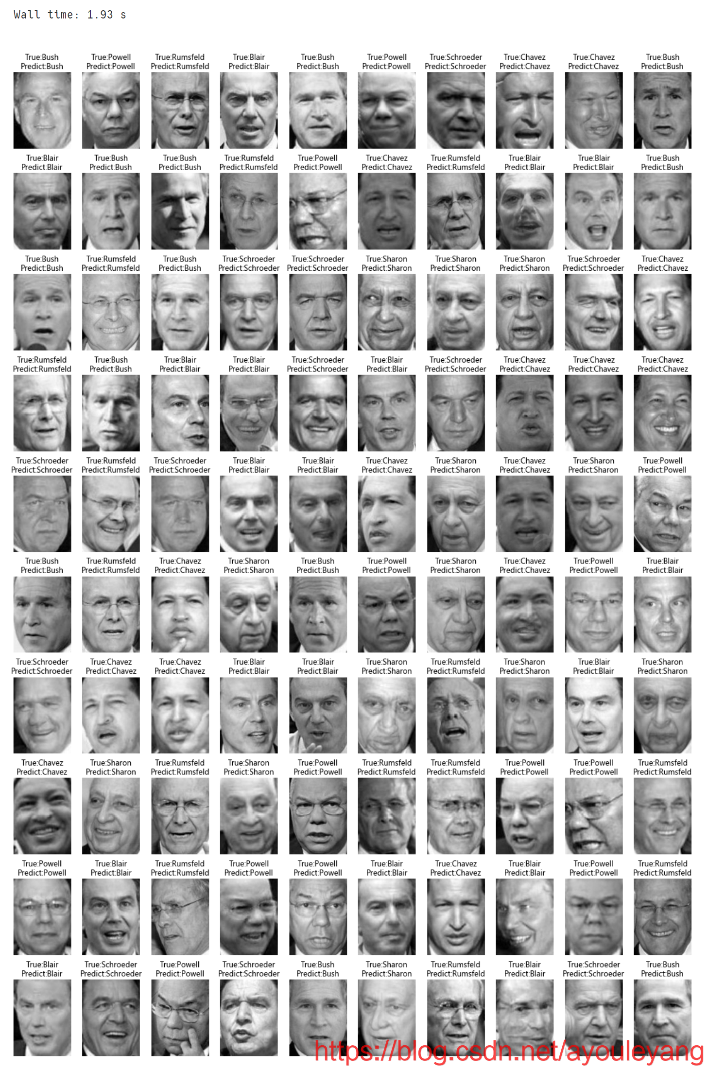

作者：阿优乐扬

链接：https://blog.csdn.net/ayouleyang/article/details/105045254

来源：CSDN
著作权归作者所有，转载请联系作者获得授权，切勿私自转载。